The impact of the state on pricing processes
7. Marketing decisions on pricing 7.1.
In general, an automatic system consists of a control object and a set of devices that provide control of this object. As a rule, this set of devices includes measuring devices, amplifying and converting devices, as well as actuators. If we combine these devices into one link (control device), then the block diagram of the system looks like this:
In an automatic system, information about the state of the control object is supplied to the input of the control device through a measuring device. Such systems are called feedback systems or closed systems. The absence of this information in the control algorithm indicates that the system is open. We will describe the state of the control object at any time  variables
  , which are called system coordinates or state variables. It is convenient to consider them as coordinates
  - dimensional state vector.
The measuring device provides information about the state of the object. If based on the vector measurement  the values of all coordinates can be found
  state vector
  , then the system is said to be completely observable.
The control device generates a control action  . There can be several such control actions; they form
  - dimensional control vector.
The input of the control device receives a reference input  . This input action carries information about what the state of the object should be. The control object may be subject to a disturbing influence
  , which represents a load or disturbance. Measuring the coordinates of an object is usually carried out with some errors
  , which are also random.
The task of the control device is to develop such a control action  so that the quality of functioning of the automatic system as a whole would be the best in some sense.
We will consider control objects that are manageable. That is, the state vector can be changed as required by correspondingly changing the control vector. We will assume that the object is completely observable.
For example, the position of an aircraft is characterized by six state coordinates. This  - coordinates of the center of mass,
  - Euler angles, which determine the orientation of the aircraft relative to the center of mass. The aircraft's attitude can be changed using elevators, heading, aileron and thrust vectoring. Thus the control vector is defined as follows:
 - elevator deflection angle
 - well
 - aileron
 - traction
State vector  in this case it is defined as follows:
You can pose the problem of selecting a control with the help of which the aircraft is transferred from a given initial state  to a given final state
  with minimal fuel consumption or in minimal time.
Additional complexity in solving technical problems arises due to the fact that, as a rule, various restrictions are imposed on the control action and on the state coordinates of the control object.
There are restrictions on any angle of the elevators, yaws, and ailerons:


 - traction itself is limited.
The state coordinates of the control object and their derivatives are also subject to restrictions that are associated with permissible overloads.
We will consider control objects that are described by the differential equation:

 (1)
(1)
Or in vector form:

 -
- -dimensional vector of object state
 -
- -dimensional vector of control actions
 - function of the right side of equation (1)
To the control vector  a restriction is imposed, we will assume that its values belong to some closed region
  some
some  -dimensional space. This means that the executive function
  belongs to the region at any time
  (
( ).
).
So, for example, if the coordinates of the control function satisfy the inequalities:


then the area  is
is  -measured cube.
Let us call any piecewise continuous function an admissible control  , whose values at each moment of time
  belongs to the region
  , and which may have discontinuities of the first kind. It turns out that even in some optimal control problems the solution can be obtained in the class of piecewise continuous control. To select control
  as a function of time and initial state of the system
  , which uniquely determines the movement of the control object, it is required that the system of equations (1) satisfy the conditions of the theorem of existence and uniqueness of the solution in the area
  . This area contains possible trajectories of the object’s movement and possible control functions.
  . If the domain of variation of variables is convex, then for the existence and uniqueness of a solution it is sufficient that the function
 . were continuous in all arguments and had continuous partial derivatives with respect to variables
 .
.
As a criterion that characterizes the quality of system operation, a functional of the form is selected:
 (2)
(2)
As a function  we will assume that it is continuous in all its arguments and has continuous partial derivatives with respect to
 .
.
In recent years, optimal management has begun to be used both in technical systems to improve the efficiency of production processes, and in organizational management systems to improve the activities of enterprises, organizations, and sectors of the national economy.
In organizational systems, one is usually interested in the final, established result of the team, without exploring
efficiency during the transition process between issuing a command and obtaining the final result. This is explained by the fact that usually in such systems the losses in the transition process are quite small and do not significantly affect the overall gain in the steady state, since the steady state itself is much longer than the transition process. But sometimes dynamics are not studied due to mathematical difficulties. Courses of methods are devoted to methods for optimizing final states in organizational and economic systems. optimization and operations research.
In the control of dynamic technical systems, optimization is often essential specifically for transient processes, in which the efficiency indicator depends not only on the current coordinate values (as in extreme control), but also on the nature of the change in the past, present and future, and is expressed by some functional on the coordinates, their derivatives and, perhaps, time.
An example is the control of an athlete running over a distance. Since his energy reserve is limited by physiological factors, and the consumption of the reserve depends on the nature of the run, the athlete can no longer give the maximum possible power at each moment, so as not to use up the energy reserve prematurely and not run out of energy over the distance, but must look for the optimal running mode for his characteristics .
Finding optimal control in such dynamic problems requires solving a rather complex mathematical problem in the control process using the methods of calculus of variations or mathematical programming, depending on the type of mathematical description (mathematical model) of the system. Thus, the calculating device or computer becomes an organic component of the optimal control system. The principle is explained in Fig. 1.10. The input of the computing device (machine) VM receives information about the current values of coordinates x from the output of the object O, about controls and from its input, about external influences z on the object, as well as setting various conditions from the outside: the value of the optimality criterion for boundary conditions, information about permissible values Computing
6.2.1. Statement and classification of problems in optimal control theory. In the overwhelming majority of the problems we considered, factors associated with changes in the objects and systems under study over time were taken out of the equation. Perhaps, if certain prerequisites are met, such an approach is constructive and legitimate. However, it is also obvious that this is not always acceptable. There is a wide class of problems in which it is necessary to find the optimal actions of an object, taking into account the dynamics of its states in time and space. Methods for solving them are the subject of the mathematical theory of optimal control.
In a very general form, the optimal control problem can be formulated as follows:
There is a certain object, the state of which is characterized by two types of parameters - state parameters and control parameters, and depending on the choice of the latter, the process of managing the object proceeds in one way or another. The quality of the control process is assessed using a certain functional*, on the basis of which the task is set: to find a sequence of values of control parameters for which this functional takes an extreme value.
* Functionality is a numerical function whose arguments, as a rule, are other functions.
From a formal point of view, many optimal control problems can be reduced to high-dimensional linear or nonlinear programming problems, since each point in the state space has its own vector of unknown variables. Still, as a rule, movement in this direction without taking into account the specifics of the corresponding problems does not lead to rational and effective algorithms for solving them. Therefore, methods for solving optimal control problems are traditionally associated with other mathematical apparatus, originating from the calculus of variations and the theory of integral equations. It should also be noted that, again, for historical reasons, the theory of optimal control was focused on physical and technical applications, and its application to solve economic problems is, in a certain sense, of a secondary nature. At the same time, in a number of cases, research models using the apparatus of optimal control theory can lead to meaningful and interesting results.
To the above, it is necessary to add a remark about the close connection that exists between the methods used to solve optimal control problems and dynamic programming. In some cases they can be used on an alternative basis, and in others they can complement each other quite successfully.
There are various approaches to classifying optimal control problems. First of all, they can be classified depending on the control object:
Ø Ø management tasks with lumped parameters;
Ø Ø object management tasks with distributed parameters.
An example of the former is the control of an aircraft as a whole, and the latter is the control of a continuous technological process.
Depending on the type of outcomes to which the applied controls lead, there are deterministic And stochastic tasks. In the latter case, the result of control is a set of outcomes described by the probabilities of their occurrence.
Based on the nature of changes in the controlled system over time, tasks are distinguished:
Ø Ø with discrete changing times;
Ø Ø with continuously changing times.
Problems of managing objects with a discrete or continuous set of possible states are classified similarly. Control problems for systems in which time and states change discretely are called control problems finite state machines. Finally, under certain conditions, problems of managing mixed systems can be set.
Many models of controlled systems are based on the apparatus of differential equations, both ordinary and partial derivatives. When studying systems with distributed parameters, depending on the type of partial differential equations used, such types of optimal control problems are distinguished as parabolic, elliptic or hyperbolic.
Let's consider two simple examples of problems of managing economic objects.
Resource allocation problem. Available T warehouses with numbers i (i∊1:m), intended for storing a homogeneous product. At discrete moments in time t∊0:(T-l) it is distributed between consumer objects (clients) with numbers j, j∊1:n. Replenishment of stock at product storage points in t- instant of time is determined by the quantities a i t,i∊1:m, and customer needs for it are equal b j t, j∊1:n. Let us denote by c t i,j- the cost of delivering a unit of product from i th warehouse j-th consumer at time t. It is also assumed that the product received at the warehouse at the time t, can be used starting from the next moment ( t+l). For the formulated model, the task is to find such a resource distribution plan ( x t i,j} Tm x n, which minimizes the total costs of delivering products to consumers from warehouses during the full period of operation of the system.
Designated by x t i,j quantity of product supplied j-th client with i th warehouse in t th moment of time, and after z t i- total quantity of product per i warehouse, the problem described above can be represented as the problem of finding such sets of variables
which minimize the function

under conditions

where is the volume of initial product inventories in warehouses z 0 i = ži. are assumed to be given.
Problem (6.20)-(6.23) is called dynamic transport linear programming problem. In terms of the above terminology, independent variables x t i,j represent control parameters system, and the variables that depend on them z t i- totality state parameters systems at any given time t. Restrictions z t i≥ 0 guarantee that at any moment in time a volume of product exceeding its actual quantity cannot be exported from any warehouse, and restrictions (6.21) set the rules for changing this quantity when moving from one period to another. Constraints of this type, which set conditions on the values of the system state parameters, are usually called phase.
Note also that condition (6.21) serves as the simplest example of phase restrictions, since the values of state parameters for two adjacent periods are associated t And t+l. In general, a dependency can be established for a group of parameters belonging to several, possibly non-contiguous, stages. Such a need may arise, for example, when taking into account the delivery delay factor in models.
The simplest dynamic model of macroeconomics. Let us imagine the economy of a certain region as a set P industries ( j∊1:P), the gross product of which in monetary terms at some point t can be represented as a vector z t=(z t 1 , z t 2 ,..., z t n), Where t∊0:(T-1). Let us denote by A t matrix of direct costs, the elements of which a t i,j, reflect product costs i th industry (in monetary terms) for the production of a unit of product j-th industry in t th moment in time. If Xt= ║x t i,j║n x m- matrix specifying specific production standards i-industry going to expand production in j-th industry, and y t = (y t 1 , y t 2 , ..., y t n) is the vector of volumes of products of consumer sectors going for consumption, then the condition of expanded reproduction can be written as
Where z 0 = ž - the initial stock of products of the industries is assumed to be given and
In the model under consideration, the quantities z t are parameters of the system state, and Xt- control parameters. On its basis, various tasks can be posed, a typical representative of which is the problem of optimal output of the economy at the moment T to some given state z*. This problem comes down to finding a sequence of control parameters

satisfying conditions (6.24)-(6.25) and minimizing the function
6.2.2. The simplest optimal control problem. One of the techniques used to solve extremal problems is to isolate a certain problem that admits of a relatively simple solution, to which other problems can be reduced in the future.
Let's consider the so-called the simplest control problem. She looks like

The specificity of the conditions of the problem (6.27)-(6.29) is that the control quality functions (6.27) and restrictions (6.28) are linear with respect to z t, at the same time function g(t, x t), included in (6.28), can be arbitrary. The last property makes the problem nonlinear even with t=1, i.e. in the static version.
The general idea of solving problem (6.27)-(6.29) comes down to “splitting” it into subtasks for each individual moment in time, under the assumption that they are successfully solvable. Let us construct the Lagrange function for problem (6.27)-(6.29)

where λ t- vector of Lagrange multipliers ( t∊0:T). Restrictions (6.29), which are of a general nature, are not included in function (6.30) in this case. Let's write it in a slightly different form

Necessary conditions for the extremum of the function Ф (x, z,λ) over a set of vectors z t are given by a system of equations
which is called system for conjugate variables. As you can see, the process of finding parameters λ t in system (6.32) is carried out recursively in the reverse order.
Necessary conditions for the extremum of the Lagrange function in the variables λ t will be equivalent to restrictions (6.28), and, finally, the conditions for its extremum over a set of vectors x t∊X t, t∊1:(T-1) must be found as a result of solving the problem
Thus, the problem of finding an optimal control is reduced to searching for controls that are suspected of being optimal, i.e., those for which the necessary optimality condition is satisfied. This, in turn, comes down to finding such t, t, t, satisfying the system of conditions (6.28), (6.32), (6.33), which is called Pontryagin's discrete maximum principle.
The theorem is true.
Proof.
Let t, t, t, satisfy system (6.28), (6.32), (6.33). Then from (6.31) and (6.32) it follows that

and since t satisfies (6.33), then
On the other hand, by virtue of (6.28) it follows from (6.30) that for any vector t
Hence,
Applying theorem (6.2), as well as the provisions of the theory of nonlinear programming concerning the connection between the solution of an extremal problem and the existence of a saddle point (see section 2.2.2), we come to the conclusion that the vectors t, t are the solution to the simplest optimal control problem (6.27)-(6.29).
As a result, we received a logically simple scheme for solving this problem: from relations (6.32) the conjugate variables are determined t, then in the course of solving problem (6.33) the controls are found t and further from (6.28) - the optimal trajectory of states t,.
The proposed method relates to the fundamental results of the theory of optimal control and, as mentioned above, is important for solving many more complex problems, which, one way or another, are reduced to the simplest. At the same time, the limits of its effective use are obvious, which entirely depend on the possibility of solving problem (6.33).
KEY CONCEPTS
Ø Ø Game, player, strategy.
Ø Ø Zero-sum games.
Ø Ø Matrix games.
Ø Ø Antagonistic games.
Ø Ø Principles of maximin and minimax.
Ø Ø Saddle point of the game.
Ø Ø Game price.
Ø Ø Mixed strategy.
Ø Ø Main theorem of matrix games.
Ø Ø Dynamic transport problem.
Ø Ø The simplest dynamic model of macroeconomics.
Ø Ø The simplest optimal control problem.
Ø Ø Pontryagin's discrete maximum principle.
CONTROL QUESTIONS
6.1. Briefly formulate the subject of game theory as a scientific discipline.
6.2. What is the meaning of the concept “game”?
6.3. To describe what economic situations can the apparatus of game theory be used?
6.4. What game is called antagonistic?
6.5. How are matrix games uniquely defined?
6.6. What are the principles of maximin and minimax?
6.7. Under what conditions can we say that a game has a saddle point?
6.8. Give examples of games that have a saddle point and those that do not.
6.9. What approaches exist to determining optimal strategies?
6.10. What is called the “price of the game”?
6.11. Define the concept of “mixed strategy”.
BIBLIOGRAPHY
1. Abramov L. M., Kapustin V. F. Mathematical programming. L., 1981.
2. Ashmanov S. A. Linear programming: Textbook. allowance. M., 1981.
3. Ashmanov S. A., Tikhonov A. V. Optimization theory in problems and exercises. M., 1991.
4. Bellman R. Dynamic programming. M., 1960.
5. Bellman R., Dreyfus S. Applied problems of dynamic programming. M., 1965.
6. Gavurin M.K., Malozemov V.N. Extremal problems with linear constraints. L., 1984.
7. Gass S. Linear programming (methods and applications). M., 1961.
8. Gail D. Theory of linear economic models M., 1963.
9. Gill F., Murray W., Wright M. Practical optimization / Transl. from English M., 1985.
10. Davydov E. G. Operations Research: Proc. manual for university students. M., 1990.
11. Danzig J. Linear programming, its generalizations and applications. M., 1966.
12. Eremin I. I., Astafiev N. N. Introduction to the theory of linear and convex programming. M., 1976.
13. Ermolyev Yu.M., Lyashko I.I., Mikhalevich V.S., Tyuptya V.I. Mathematical methods of operations research: Proc. manual for universities. Kyiv, 1979.
14. Zaichenko Yu. P. Operations Research, 2nd ed. Kyiv, 1979.
15. Zangwill W. I. Nonlinear programming. Unified approach. M., 1973.
16. Zeutendijk G. Methods of possible directions. M., 1963.
17. Karlin S. Mathematical methods in game theory, programming and economics. M., 1964.
18. Karmanov V. G. Mathematical programming: Textbook. allowance. M., 1986.
19. Korbut A.A., Finkelyitein Yu.Yu. Discrete programming. M., 1968.
20. Kofman A., Henri-Laborder A. Operations research methods and models. M., 1977.
21. Kuntze G.P., Krelle V. Nonlinear programming. M., 1965.
22. Lyashenko I.N., Karagodova E.A., Chernikova N.V., Shor N.3. Linear and nonlinear programming. Kyiv, 1975.
23. McKinsey J. Introduction to game theory. M., 1960.
24. Mukhacheva E. A., Rubinshtein G. Sh. Mathematical programming. Novosibirsk, 1977.
25. Neumann J., Morgenstern O. Game theory and economic behavior. M, 1970.
26. Ore O. Graph theory. M., 1968.
27. Taha X. Introduction to Operations Research / Trans. from English M., 1985.
28. Fiacco A., McCormick G. Nonlinear programming. Methods of sequential unconditional minimization. M., 1972.
29. Hadley J. Nonlinear and dynamic programming. M., 1967.
30. Yudin D.B., Golshtein E.G. Linear programming (theory, methods and applications). M., 1969.
31. Yudin D.B., Golshtein E.G. Linear programming. Theory and final methods. M., 1963.
32. Lapin L. Quantitative methods for business decisions with cases. Fourth edition. HBJ, 1988.
33. Liitle I.D.C., Murty K.G., Sweeney D.W., Karel C. An algorithm for traveling for the traveling salesman problem. - Operation Research, 1963, vol.11, No. 6, p. 972-989/ Russian. translation: Little J., Murthy K., Sweeney D., Kerel K. Algorithm for solving the traveling salesman problem. - In the book: Economics and mathematical methods, 1965, vol. 1, no. 1, p. 94-107.
PREFACE................................................... ........................................................ ........................................................ ........................................................ ..... 2
INTRODUCTION........................................................ ........................................................ ........................................................ ........................................................ ............. 3
CHAPTER 1. LINEAR PROGRAMMING.................................................... ........................................................ ........................................... 8
1.1. FORMULATION OF THE LINEAR PROGRAMMING PROBLEM.................................................................... ............................................... 9
1.2. BASIC PROPERTIES OF ZLP AND ITS FIRST GEOMETRIC INTERPRETATION................................................................... ................. eleven
1.3. BASIC SOLUTIONS AND SECOND GEOMETRICAL INTERPRETATION OF THE ZLP................................................................... .......................... 15
1.4. SIMPLEX METHOD................................................... ........................................................ ........................................................ .................................... 17
1.5. MODIFIED SIMPLEX METHOD.................................................................... ........................................................ .................................... 26
1.6. THEORY OF DUALITY IN LINEAR PROGRAMMING.................................................... .......................................... thirty
1.7. DUAL SIMPLEX METHOD.................................................... ........................................................ ........................................................ .37
KEY CONCEPTS................................................................... ........................................................ ........................................................ ........................................... 42
CONTROL QUESTIONS................................................ ........................................................ ........................................................ ........................... 43
CHAPTER 2. NONLINEAR PROGRAMMING.................................................... ........................................................ .................................... 44
2.1. METHODS FOR SOLVING NONLINEAR PROGRAMMING PROBLEMS.................................................... ........................................... 44
2.2. DUALITY IN NONLINEAR PROGRAMMING.................................................................... ........................................................ ...55
KEY CONCEPTS................................................................... ........................................................ ........................................................ .................................... 59
CONTROL QUESTIONS................................................ ........................................................ ........................................................ ........................... 59
CHAPTER 3. TRANSPORT AND NETWORK TASKS.................................................... ........................................................ ................................... 60
3.1. TRANSPORT PROBLEM AND METHODS OF ITS SOLUTION.................................................... ........................................................ ........................... 60
3.2. NETWORK TASKS................................................................ ........................................................ ........................................................ ..................................... 66
KEY CONCEPTS................................................................... ........................................................ ........................................................ .................................... 73
CONTROL QUESTIONS................................................ ........................................................ ........................................................ ........................... 73
CHAPTER 4. DISCRETE PROGRAMMING.................................................... ........................................................ .................................... 74
4.1. TYPES OF DISCRETE PROGRAMMING TASKS.................................................................. ........................................................ .................... 74
4.2. GOMORI METHOD................................................... ........................................................ ........................................................ ........................................... 78
4.3. BRANCH AND BOUNDS METHOD.................................................... ........................................................ ........................................................ ........................ 81
KEY CONCEPTS................................................................... ........................................................ ........................................................ .................................... 86
CONTROL QUESTIONS................................................ ........................................................ ........................................................ ........................... 86
CHAPTER 5. DYNAMIC PROGRAMMING.................................................... ........................................................ ............................ 86
5.1. GENERAL SCHEME OF DYNAMIC PROGRAMMING METHODS.................................................................... .................................... 86
5.2. EXAMPLES OF DYNAMIC PROGRAMMING PROBLEMS.................................................................... ........................................................ .... 93
KEY CONCEPTS................................................................... ........................................................ ........................................................ .................................... 101
CONTROL QUESTIONS................................................ ........................................................ ........................................................ ............................... 101
CHAPTER 6. BRIEF OVERVIEW OF OTHER SECTIONS OF OPERATIONS RESEARCH................................................... ........................ 101
6.1. GAME THEORY................................................ ........................................................ ........................................................ ........................................................ 101
6.2. OPTIMAL CONTROL THEORY.................................................... ........................................................ ........................................... 108
KEY CONCEPTS................................................................... ........................................................ ........................................................ .................................... 112
CONTROL QUESTIONS................................................ ........................................................ ........................................................ ............................... 112
BIBLIOGRAPHY................................................ ........................................................ ........................................................ .................................... 112
Optimal control
Optimal control is the task of designing a system that provides, for a given control object or process, a control law or a control sequence of influences that ensures the maximum or minimum of a given set of system quality criteria.
To solve the optimal control problem, a mathematical model of the controlled object or process is constructed, describing its behavior over time under the influence of control actions and its own current state. The mathematical model for the optimal control problem includes: the formulation of the control goal, expressed through the control quality criterion; determination of differential or difference equations describing possible ways of movement of the control object; determination of restrictions on the resources used in the form of equations or inequalities.
The most widely used methods in the design of control systems are the calculus of variations, Pontryagin's maximum principle and Bellman dynamic programming.
Sometimes (for example, when managing complex objects, such as a blast furnace in metallurgy or when analyzing economic information), the initial data and knowledge about the controlled object when setting the optimal control problem contains uncertain or fuzzy information that cannot be processed by traditional quantitative methods. In such cases, you can use optimal control algorithms based on the mathematical theory of fuzzy sets (Fuzzy control). The concepts and knowledge used are converted into fuzzy form, fuzzy rules for deriving decisions are determined, and then the fuzzy decisions are converted back into physical control variables.
Let us formulate the optimal control problem:
here is the state vector - control, - the initial and final moments of time.
The optimal control problem is to find state and control functions for time that minimize the functionality.
Let us consider this optimal control problem as a Lagrange problem in the calculus of variations. To find the necessary conditions for an extremum, we apply the Euler-Lagrange theorem. The Lagrange function has the form: , where are the boundary conditions. The Lagrangian has the form: , where , , are n-dimensional vectors of Lagrange multipliers.
The necessary conditions for an extremum, according to this theorem, have the form:
Necessary conditions (3-5) form the basis for determining optimal trajectories. Having written these equations, we obtain a two-point boundary problem, where part of the boundary conditions is specified at the initial moment of time, and the rest at the final moment. Methods for solving such problems are discussed in detail in the book.
The need for the Pontryagin maximum principle arises in the case when nowhere in the admissible range of the control variable is it possible to satisfy the necessary condition (3), namely .
In this case, condition (3) is replaced by condition (6):
(6)In this case, according to Pontryagin's maximum principle, the value of optimal control is equal to the value of control at one of the ends of the admissible range. Pontryagin's equations are written using the Hamilton function H, defined by the relation. From the equations it follows that the Hamilton function H is related to the Lagrange function L as follows: . Substituting L from the last equation into equations (3-5) we obtain the necessary conditions expressed through the Hamilton function:
Necessary conditions written in this form are called Pontryagin equations. Pontryagin's maximum principle is discussed in more detail in the book.
The maximum principle is especially important in control systems with maximum speed and minimum energy consumption, where relay-type controls are used that take extreme rather than intermediate values within the permissible control interval.
For the development of the theory of optimal control L.S. Pontryagin and his collaborators V.G. Boltyansky, R.V. Gamkrelidze and E.F. Mishchenko was awarded the Lenin Prize in 1962.
The dynamic programming method is based on Bellman's principle of optimality, which is formulated as follows: the optimal control strategy has the property that whatever the initial state and control at the beginning of the process, subsequent controls must constitute an optimal control strategy relative to the state obtained after the initial stage of the process. The dynamic programming method is described in more detail in the book
Wikimedia Foundation.
Optimal control See what “Optimal control” is in other dictionaries: - OU Control that provides the most favorable value of a certain optimality criterion (OC), characterizing the effectiveness of control under given restrictions. Various technical or economic... ...
Dictionary-reference book of terms of normative and technical documentation optimal control - Management, the purpose of which is to ensure the extreme value of the management quality indicator. [Collection of recommended terms. Issue 107. Management Theory. Academy of Sciences of the USSR. Committee of Scientific and Technical Terminology. 1984]… …
Optimal control Technical Translator's Guide - 1. The basic concept of the mathematical theory of optimal processes (belonging to the branch of mathematics under the same name: “O.u.”); means the selection of control parameters that would provide the best from the point of... ...
Allows, under given conditions (often contradictory), to achieve the goal in the best possible way, for example. in the minimum time, with the greatest economic effect, with maximum accuracy... Big Encyclopedic Dictionary
Aircraft is a section of flight dynamics devoted to the development and use of optimization methods to determine the laws of motion control of the aircraft and its trajectories that provide the maximum or minimum of the selected criterion... ... Encyclopedia of technology
A branch of mathematics that studies non-classical variational problems. Objects that technology deals with are usually equipped with “rudders”; with their help, a person controls movement. Mathematically, the behavior of such an object is described... ... Great Soviet Encyclopedia
Optimal automatic control systems are systems in which control is carried out in such a way that the required optimality criterion has an extreme value. Boundary conditions defining the initial and required final states of the system; the technological goal of the system. tн It is set in cases where the average deviation over a certain time interval is of particular interest and the task of the control system is to ensure a minimum of this integral...
If this work does not suit you, at the bottom of the page there is a list of similar works. You can also use the search button
Optimal control
Voronov A.A., Titov V.K., Novogranov B.N. Fundamentals of the theory of automatic regulation and control. M.: Higher School, 1977. 519 p. P. 477 491.
Optimal self-propelled guns these are systems in which control is carried out in such a way that the required optimality criterion has an extreme value.
Examples of optimal object management:
The optimal control problem is formulated as follows:
“Find such a law of change in control time
u(t ), in which the system, under given restrictions, will move from one given state to another in an optimal way in the sense that the functional I , expressing the quality of the process, will receive an extreme value “.To solve the optimal control problem, you need to know:
1. Mathematical description of the object and environment, connecting the values of all coordinates of the process under study, control and disturbing influences;
2. Physical restrictions on coordinates and control law, expressed mathematically;
3. Boundary conditions defining the initial and required final states of the system
(technological goal of the system);
4. Objective function (quality functional
mathematical goal).
Mathematically, the optimality criterion is most often presented as:
t to
I =∫ f o [ y (t), u (t), f (t), t ] dt + φ [ y (t to), t to ], (1)
t n
where the first term characterizes the quality of control over the entire interval (
tn, tn) and is calledintegral component, second term
characterizes the accuracy at the final (terminal) point in time t to .
Expression (1) is called a functional, since I depends on the choice of function u(t ) and the resulting y(t).
Lagrange problem.It minimizes functionality
t to
I=∫f o dt.
t n
It is used in cases where the average deviation over time is of particular interest.
a certain time interval, and the task of the control system is to ensure a minimum of this integral (deterioration in product quality, loss, etc.).
Examples of functionality:
I =∫ (t) dt criterion for minimum error in steady state, where x(t)
I =∫ dt = t 2 - t 1 = > min criterion for maximum speed of self-propelled guns;
I =∫ dt = > min criterion of optimal efficiency.
Mayer's problem. In this case, the functional that is minimized is the one defined only by the terminal part, i.e.
I = φ =>min.
F o (x, u, t),
you can set the following task: determine the control u (t), t n ≤ t ≤ t k so that for
given flight time to reach the maximum range, provided that at the final moment of time t to The aircraft will land, i.e. x (t to ) =0.
Boltz problem reduces to the problem of minimizing criterion (1).
The basic methods for solving optimal control problems are:
1.Classical calculus of variations Euler’s theorem and equation;
2. The principle of maximum L.S. Pontryagin;
3.Dynamic programming by R. Bellman.
EULER'S EQUATION AND THEOREM
Let the functionality be given:
t to
I =∫ f o dt ,
t n
Where some twice differentiable functions, among which it is necessary to find such functions ( t ) or extremals , which satisfy the given boundary conditions x i (t n), x i (t k ) and minimize functionality.
Extremals are found among solutions of the Euler equation
I = .
To establish the fact of minimizing the functional, it is necessary to make sure that the Lagrange conditions are satisfied along the extremals:
similar to the requirements for the positivity of the second derivative at the minimum point of the function.
Euler's theorem: “If the extremum of the functional I exists and is achieved among smooth curves, then it can only be achieved on extremals.”
L.S.PONTRYAGIN’S MAXIMUM PRINCIPLE
The school of L.S. Pontryagin formulated a theorem about the necessary condition of optimality, the essence of which is as follows.
Let us assume that the differential equation of the object, together with the unchangeable part of the control device, is given in the general form:
To control u j restrictions may be imposed, for example, in the form of inequalities:
, .
The purpose of control is to transfer the object from the initial state ( t n ) to the final state ( t to ). The end of the process t to may be fixed or free.
Let the optimality criterion be the minimum of the functional
I = dt.
Let's introduce auxiliary variables and form a function
Fo ()+ f () f ()+
The maximum principle states that for the system to be optimal, i.e. to obtain the minimum of the functional, it is necessary to exist such non-zero continuous functions satisfying the equation
That for any t , located in a given range t n≤ t ≤ t k , the value of H, as a function of admissible control, reaches a maximum.
The maximum of the function H is determined from the conditions:
if it does not reach the boundaries of the region, and as the supremum of the function H, otherwise.
Dynamic programming by R. Bellman
R. Bellman's principle of optimality:
“Optimal behavior has the property that, whatever the initial state and decision at the initial moment, subsequent decisions must constitute optimal behavior relative to the state resulting from the first decision.”
The “behavior” of the system should be understood movement these systems, and the term"decision" refers tothe choice of the law of change in time of control forces.
In dynamic programming, the process of searching for extremals is divided into n steps, while in the classical calculus of variations the search for the entire extremal is carried out.
The process of searching for an extremal is based on the following premises of R. Bellman’s optimality principle:
Heuristically, the Bellman equations for the required problem statements are derived for continuous and discrete systems.
Adaptive Control
Andrievsky B.R., Fradkov A.L. Selected chapters of automatic control theory with examples in language MATLAB . St. Petersburg: Nauka, 1999. 467 p. Chapter 12.
Voronov A.A., Titov V.K., Novogranov B.N. Fundamentals of the theory of automatic regulation and control. M.: Higher School, 1977. 519 p. P. 491 499.
Ankhimyuk V.L., Opeiko O.F., Mikheev N.N. Theory of automatic control. Mn.: Design PRO, 2000. 352 p. P. 328 340.
The need for adaptive control systems arises due to the significant complication of the control problems being solved, and a specific feature of this complication is the lack of practical opportunity for a detailed study and description of the processes occurring in the controlled object.
For example, modern high-speed aircraft, accurate a priori data on the characteristics of which under all operating conditions cannot be obtained due to significant variations in atmospheric parameters, large ranges of flight speeds, ranges and altitudes, as well as due to the presence of a wide range of parametric and external disturbances.
Some control objects (aircraft and missiles, technological processes and power plants) are distinguished by the fact that their static and dynamic characteristics change over a wide range in a manner that was not anticipated in advance. Optimal management of such objects is possible with the help of systems in which the missing information is automatically replenished by the system itself during operation.
Adaptive (lat.) adaptio ” device) are those systems that, when changing the parameters of objects or the characteristics of external influences during operation, independently, without human intervention, change the parameters of the regulator, its structure, settings or regulatory influences to maintain the optimal operating mode of the object.
The creation of adaptive control systems is carried out in fundamentally different conditions, i.e. adaptive methods should help achieve high quality control in the absence of sufficient completeness of a priori information about the characteristics of the controlled process or in conditions of uncertainty.
Classification of adaptive systems:
Self-adapting
(adaptive)
Control systems
Self-adjusting Self-learning Systems with adaptation
Systems systems in special phases
States
Search Searchless- Training- Training- Relay Adaptive
(extreme (analysed with incentives without self-oscillation system with
New) tic incentive variables
Systems systems systems structure
Structural diagram of AS classification (according to the nature of the adaptation process)
Self-tuning systems (SNS)are systems in which adaptation to changing operating conditions is carried out by changing parameters and control actions.
Self-organizingThese are systems in which adaptation is carried out by changing not only parameters and control actions, but also the structure.
Self-learningthis is an automatic control system in which the optimal operating mode of the controlled object is determined using a control device, the algorithm of which is automatically purposefully improved in the learning process through automatic search. The search is carried out using a second control device, which is an organic part of the self-learning system.
In search engines systems, changing the parameters of the control device or control action is carried out as a result of searching for conditions for the extremum of quality indicators. The search for extremum conditions in systems of this type is carried out using test influences and assessmentobtained results.
In non-search systems, the determination of the parameters of the control device or control actions is carried out on the basis of the analytical determination of the conditions that ensure the specified quality of control without the use of special search signals.
Systems with adaptation in special phase statesuse special modes or properties of nonlinear systems (self-oscillation modes, sliding modes) to organize controlled changes in the dynamic properties of the control system. Specially organized special modes in such systems either serve as an additional source of operational information about the changing operating conditions of the system, or endow the control systems with new properties, due to which the dynamic characteristics of the controlled process are maintained within the desired limits, regardless of the nature of the changes that arise during operation.
When using adaptive systems, the following main tasks are solved:
1 . During the operation of the control system, when parameters, structure and external influences change, control is provided in which the specified dynamic and static properties of the system are maintained;
2 . During the design and commissioning process, in the initial absence of complete information about the parameters, structure of the control object and external influences, the system is automatically adjusted in accordance with the specified dynamic and static properties.
Example 1 . Adaptive aircraft angular position stabilization system.
f 1 (t) f 2 (t) f 3 (t)
D1 D2 D3
VU1 VU2 VU3 f (t) f 1 (t) f 2 (t) f 3 (t)
u (t) W 1 (p) W 0 (p) y (t)
+ -
Rice. 1.
Adaptive aircraft stabilization system
When flight conditions change, the transfer function changes W 0 (p ) aircraft, and, consequently, the dynamic characteristics of the entire stabilization system:
. (1)
Disturbances from the external environment f 1 (t), f 2 (t), f 3 (t ) , leading to controlled changes in system parameters, are applied to various points of the object.
Disturbing influence f(t ) applied directly to the input of the control object, in contrast to f 1 (t), f 2 (t), f 3 (t ) does not change its parameters. Therefore, during system operation, only f 1 (t), f 2 (t), f 3 (t).
In accordance with the feedback principle and expression (1), uncontrolled changes in characteristics W 0 (p ) due to disturbances and interference cause relatively small changes in the parameters Ф( p) .
If we set the task of more complete compensation of controlled changes, so that the transfer function Ф(р) of the aircraft stabilization system remains practically unchanged, then the characteristic of the controller should be changed appropriately W 1 (p ). This is done in an adaptable self-propelled gun, made according to the scheme in Fig. 1. Environmental parameters characterized by signals f 1 (t), f 2 (t), f 3 (t ), for example, velocity head pressure P H(t) , ambient temperature T0(t) and flight speed v(t) , are continuously measured by sensors D 1, D 2, D 3 , and the current parameter values are sent to computing devices B 1, B 2, B 3 , producing signals with the help of which the characteristic is adjusted W 1 (p ) to compensate for changes in characteristics W0(p).
However, in an automated control system of this type (with an open configuration loop) there is no self-analysis of the effectiveness of the controlled changes it makes.
Example 2. Extreme aircraft flight speed control system.
Z Disturbance
Impact
X 3 = X 0 - X 2
Automatic device X 0 Amplification X 4 Executive X 5 Adjustable X 1
Mathematical converter device object
Extremum iska + - device
Measuring
Device
Fig. 2. Functional diagram of an extreme aircraft flight speed control system
The extremal system determines the most profitable program, i.e. then the value X 1 (required speed of the aircraft), which must be maintained at the moment in order to produce a minimum fuel consumption per unit path length.
Z - characteristics of the object; X 0 - control influence on the system.
(fuel consumption value)
y(0)
y(T)
Self-organizing systems
These standards separately normalize each component of the microclimate in the working area of the production premises: temperature, relative humidity, speed of air movement, depending on the ability of the human body to acclimatize at different times of the year, the nature of clothing, the intensity of the work performed and the nature of heat generation in the work area. Changes in air temperature in height and horizontally, as well as changes in air temperature during a shift while ensuring optimal microclimate values in the workplace should not... Management: concept, features, system and principles Government bodies: concept, types and functions. In terms of content, administrative law is public-administrative law that realizes the legal interests of the majority of citizens, for which the subjects of management are endowed with legally authoritative powers and representative functions of the state. Consequently, the object of action of legal norms are specific managerial social relations that arise between the subject of management by the manager and the objects... State regulation of the socio-economic development of regions. Local budgets as the financial basis for the socio-economic development of the region. Different territories of Ukraine have their own characteristics and differences both in terms of economic development and in social, historical, linguistic and mental aspects. Of these problems, we must first of all mention the imperfection of the sectoral structure of most regional economic complexes; their low economic efficiency; significant differences between regions in levels...
7. Marketing decisions on pricing 7.1.

Grilled chicken in the oven. What could be simpler and more difficult at the same time? It would seem that they took chicken, spices, turned on the oven...
Introduction 1. The concept of the marketing environment of an enterprise 1.1 The marketing environment of an enterprise, its essence and main...

Metabolism of matter and energy Metabolism of matter and energy - Metabolism Metabolism of matter and energy Metabolism is a set of processes...

Lesson topic: Raster and vector graphics.

Mini-salary: free program for calculating salaries, insurance contributions, personal income tax

Self-education


Scientific work
Presentation on the topic:

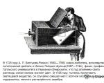
Beginning The invention of photography If you think that photography was created by one person, then you are deeply mistaken And if...
Modern society presents the legal profession as extremely prestigious and well-paid. Hollywood...
Controlling is a special concept of enterprise management, which is based on a comprehensive...

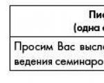
How to draw up a letter of consent correctly? Is it necessary to repeat the contents of the request letter, what to title...

Introduction 1. The concept of the marketing environment of an enterprise 1.1 The marketing environment of an enterprise, its essence and main...